State of the Art Audio Classification – Simply
by Erik Tomica, Design Enterprise Studio Member, March 2021
Have you ever wondered how can humans recognise music and sounds in just a couple of seconds? And how applications like Shazam replicate that despite of such a vast amount of music released every year? How are humans able to tell someone’s emotion based on the tone of their voice and would a machine be able to do the same without any understanding of what emotion is? This post aims to answer some of these questions in a simple way. There won’t be any technical terminology and if so, this will be very simply explained so let’s dive right in:
A lot of progress in machine learning and IT in general comes from understanding humans, how we do things and why. In the case of audio recognition and audio classification we [humans] have have taken inspiration from mother nature once again. It all started with a simple question: how do we actually hear things?
How do humans perceive sound?
First things first, let’s talk about some key words:
As you may know, sound is just vibrating air and how fast it vibrates determines how “high” the sound is (in other words if the vibration is fast enough it can turn into some of those annoying high-pitched sounds around us, like neighbours’ kids crying on a Sunday morning). In a nutshell, this is a frequency measured in Hz. Most of the time when there is more than one sound you can distinguish them from each other (for example you can have a conversation with a person while hearing an ambulance in a distance). This means that sounds are transparent and there is something called amplitude measured in dB which can be explained as loudness.
This vibrating air is transferring its energy onto a membrane in our ear which translates the information to our brain (we’ve adapted this clever concept to microphones).
Now, interestingly enough, we as humans are capable of telling the difference between low frequencies quite easily and struggle with the higher ones. For example, we can tell that 400Hz is lower than 500Hz but if we hear 4400Hz and 4500Hz we just simply can’t tell which one is higher (you can try it out here, but be careful about the volume). This means that our hearing is non-linear.
Visualising the Sound
Now when we know what frequency and amplitude is, there are ways how to visualise what we hear.
If you were born before 2000’ you might probably remember Microsoft’s media player. It was probably one of the most common player for any music, so if you’ve owned a CD of your favourite band and a PC there is a big chance you used this software. Part of it was this unique visual of music which was changing with the music and looked like this:


These visuals come from a process called Fast-Fourier Transform – FFT. We are not going to discuss the details of what it is, for our purposes it is enough to just know that FFT is an algorithm that can help us determine amplitude of a given frequencies at any given time. This is nicely represented in the picture on the left the x-axis represents different frequencies and the y-axis represents their amplitudes.
You can do a lot of creative things with FFT alone and the vast majority of ‘cool’ looking visuals that accompany music are visualised results of FFT. This is only a two-dimensional image but we can even go to the 3rd dimension!
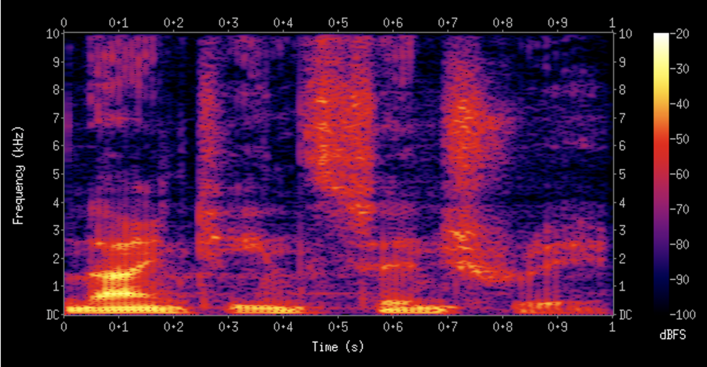
Another form of visualising sound is a spectrogram – similar to the previous examples, a spectrogram displays amplitude (in dB) and frequency (in Hz) but adds time. Spectrograms tend to look like this:

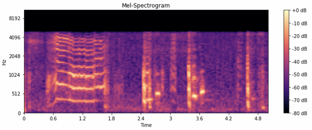
Here the colours represent the power of each frequency at any given time. But as we know, humans recognise lower frequencies much better than higher ones so it would be useful to see more details but in a different way. Luckily, someone already figured out a way of doing it and it is called Mel-powered spectrogram:

This type of spectrogram in general spreads out the lower frequencies where humans find important patterns and ‘squishes’ together the higher frequencies ones we don’t hear so well. Thanks to this technique we’ve now got ourselves a spectrogram that can be used for machine learning algorithms and sound pattern recognition!
Deep Learning Pipeline
Now let’s have a look at the machine learning side of audio classification. We will only going to focus on Deep Learning workflows here, and try to explain the state-of-the-art audio classification method which is probably going be the new standard in classifying audio.
The current focus in audio processing is (surprisingly) aimed at converting sound to image and classifying those rather than using audio itself. The reason is quite simple. A massive amount of research has already been done in image classification like face recognition or object recognition using Convolutional Neural Networks (CNN) which has made those image recognition models into extremely powerful tools. Because the aim of this post is to introduce the future of audio processing and not to explain the details of deep learning, let’s just think of CNNs as a black box full of algorithms with the ability to tweak themselves and spit out the correct class of an image (you can learn more about CNNs here).
The first step for correct audio classification then is your dataset. If building a successful classification model is like a building a house, your data are your cornerstones. The model first needs some quality information to learn from, so finding some proper audio files is essential for the model to perform well.
For example, for a recent instrument classification study I used audio files specifically meant for this task (IRMAS dataset), but the quality of the data was not overly good, so some signal processing was required to improve the accuracy. But what if you think beyond instruments? If you don’t look just for a dataset for instrument classification but rather orchestra recordings meant for creating music? London’s Philharmonia for example has such a dataset available here which is of very high quality!
The next step is to extract the correct features. I have already mentioned Mel-spectrograms which are quite simple to understand yet they can be a very powerful tool. Other feature extraction tools are FFT, STFT, MFCC and many more. We already know that FFT is showing us the amplitude of frequency at any given time and STFT (Short-Time Fourier Transform) works quite similarly.
A particularly interesting feature extraction tool are Mel-Frequency Cepstral Coefficients (MFCC) which are extremely difficult to explain (the analytic process involves windowing the signal, applying the DFT, taking the log of the magnitude, warping the frequencies on a Mel scale, followed by applying the inverse DCT). In fairly general terms they show up changes of cepstral coefficients in your audio (see full explanation of MFCCs here). This is useful, particularly for any form of voice/speech classification task.

Each of these algorithms mentioned above focus on working out something different and so in order to build a good classification model, you have to choose the correct one. Interestingly, the results of all these algorithms can be interpreted as images which are suitable for audio classification using deep learning.
Implementation and Shazam!
And so, as an example of actual use of these machine learning algorithms we have a famous application called Shazam, which works in an incredibly smart yet elegant way and can classify music in a matter of seconds. Shazam doesn’t even require a music database, so how does it work?
When you press record button in your Shazam app, it starts listening. It takes a bit of sound, converts it to our Mel-spectrogram and focuses on the peaks in the frequencies. Now imagine you draw a dot whenever there is a peak – those dots form a unique fingerprint of the audio which can be then recognised by pre-trained models and correctly labelled.
Hope you enjoyed reading about state-of-the-art audio classification techniques, if you want to know more, here is a useful youtube video explaining the whole process in a bit more in depth.
